Project Part 1

Preparing military expenditure data for plotting .

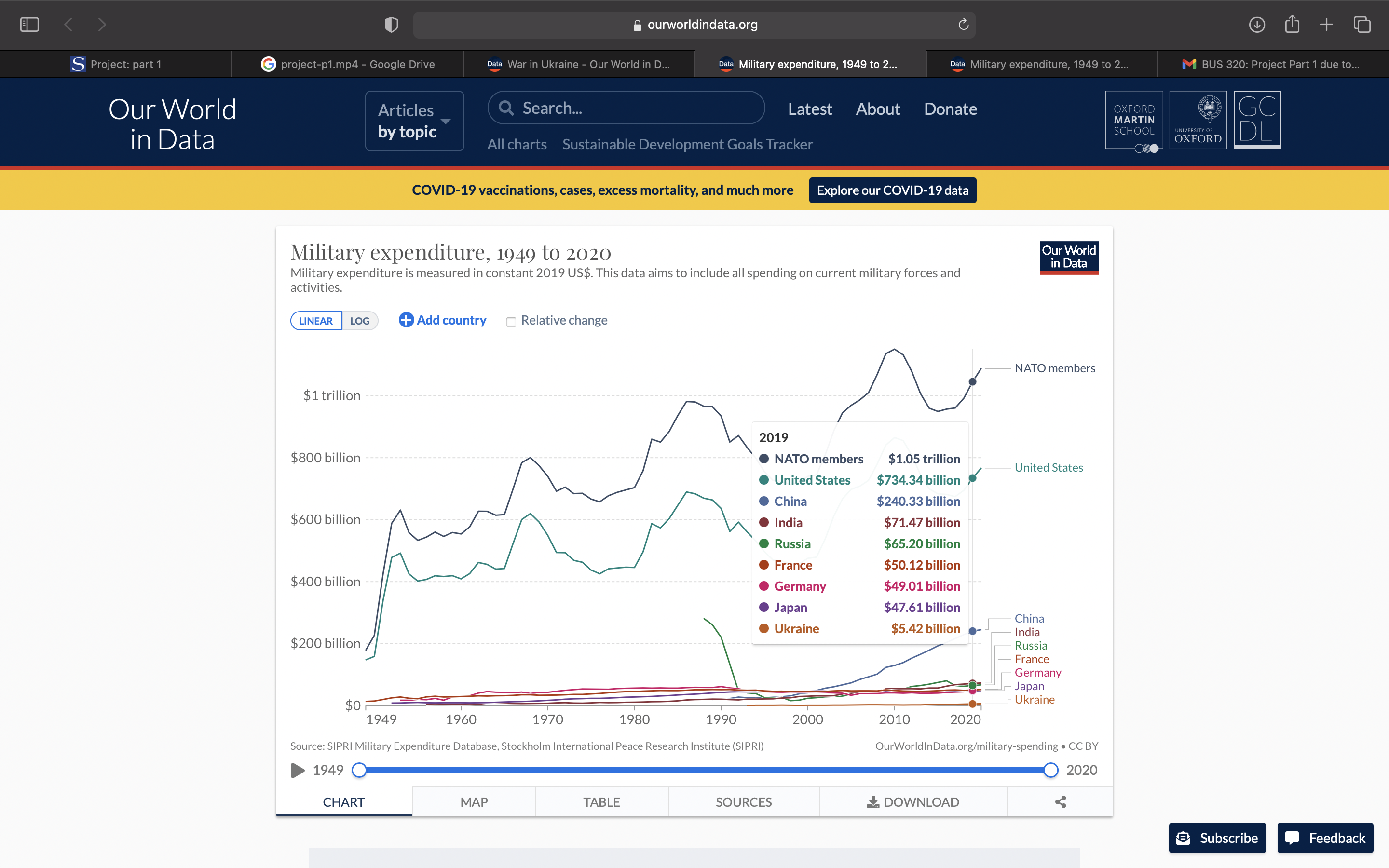
1. I download Military expenditure data across the globe from Our World in Data. I selected this data because of the war in Ukraine and the recent increase in military spending across the globe.

2. This is the Total Military Expenditure to the data.

3. The following code chunk loads the package I will use to read in and prepare the data for analysis.

library(tidyverse)

4. Read the data in

military_expenditure_total_by_region <- 
  read_csv(here::here("_posts/2022-05-08-project-part-1/military-expenditure-total.csv"))

5. Use glimpse to see the names and types of the columns.

glimpse(military_expenditure_total_by_region)

Rows: 8,278
Columns: 4
$ Entity               <chr> "Afghanistan", "Afghanistan", "Afghanis…
$ Code                 <chr> "AFG", "AFG", "AFG", "AFG", "AFG", "AFG…
$ Year                 <dbl> 1970, 1973, 1974, 1975, 1976, 1977, 200…
$ military_expenditure <dbl> 5373185, 6230685, 6056124, 6357396, 810…

6. Use output from glimpse (and view) to prepare the data for analysis

• Create the object regions that is list of regions I want to extract from the data set

• Change the name of the 1st column to Regions and 4th column to military_spending

• Use filter to extract the rows that I want to keep: Year >= 1949 and entity to Region in regions

• Select the columns to keep : Region, Year, military_spending

• Use mutate to convert military spending to millions of Dollars

• Assign output to regional_military_spending

• Display the first 8 rows of regional_military_spending

regions <- c("NATO members",
         "United States",
         "China",
         "India",
         "Russia",
         "France",
         "Japan",
         "Ukraine")

 regional_military_spending <- military_expenditure_total_by_region %>% 
   rename(Region = 1, military_spending = 4) %>% 
   filter(Year >= 1949, Region %in% regions) %>% 
   select(Region, Year, military_spending) %>% 
mutate(military_spending= military_spending*1e-9)
 
regional_military_spending

# A tibble: 442 × 3
   Region  Year military_spending
   <chr>  <dbl>             <dbl>
 1 China   1989              19.6
 2 China   1990              21.3
 3 China   1991              22.6
 4 China   1992              27.5
 5 China   1993              25.3
 6 China   1994              24.3
 7 China   1995              25.3
 8 China   1996              26.8
 9 China   1997              28.6
10 China   1998              31.2
# … with 432 more rows

Check that the total for 2019 equals in the graph

 regional_military_spending%>% filter(Year==2019) %>% 
  summarise(sum(military_spending))

# A tibble: 1 × 1
  `sum(military_spending)`
                     <dbl>
1                    2260.

Add a picture.

{width =100%}

Write the data to file to the project directory

write_csv(regional_military_spending, file = "regional_military_spending.csv")